How the distributed engine works

The Polars Nanook distributed engine runs one lazy Polars query across several workers. It splits both computation and memory, so it can process datasets larger than one machine's RAM. The open-source Polars library runs on one machine. Remote queries run on the distributed engine by default. Scale a query covers single-node execution and the number of workers a query uses.

Execution pipeline

A distributed query passes through the following pipeline:

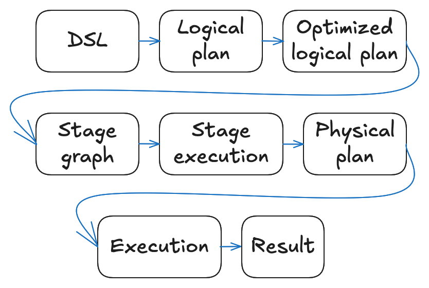
1. The query is written with the Polars DSL as a LazyFrame, translated into a logical plan (a tree of operations that describes what to compute), and rewritten by the query optimizer into an equivalent but more efficient optimized logical plan.
2. The distributed query planner walks the optimized logical plan and produces a stage graph: a DAG of stages separated by shuffles at each point where data needs to be redistributed across workers.
3. The scheduler executes stages and assigns partitions to workers in dependency order, and waits for all workers to finish a stage before it starts the next one.
4. Each worker receives the stage's part of the optimized logical plan together with its assigned partitions, derives its own physical plan, and executes it. After finishing the stage, the worker writes intermediate results to worker-local disk, a shared filesystem or object storage.
5. After the final stage, the results go to the destination location or back to the user, depending on the query.

The query profile shows the stage graph, the shuffle volume and the time spent per operator of an executed query.

Example: PDS-H query 3 on 100 GB

This example runs query 3 of the PDS-H benchmark on scale factor 100 (approx. 100GB of data) from the public datasets on the distributed engine.

import polars as pl
import polars_nanook as pn

ctx: pn.ComputeContext | pn.ClusterContext

lineitem_sf100 = pl.scan_parquet(
    "s3://polars-cloud-samples-us-east-2-prd/pdsh/sf100/lineitem/*.parquet",
    storage_options={"request_payer": "true", "aws_region": "us-east-2"},
)
customer_sf100 = pl.scan_parquet(
    "s3://polars-cloud-samples-us-east-2-prd/pdsh/sf100/customer/*.parquet",
    storage_options={"request_payer": "true", "aws_region": "us-east-2"},
)
orders_sf100 = pl.scan_parquet(
    "s3://polars-cloud-samples-us-east-2-prd/pdsh/sf100/orders/*.parquet",
    storage_options={"request_payer": "true", "aws_region": "us-east-2"},
)

def pdsh_q3(
    customer: pl.LazyFrame, lineitem: pl.LazyFrame, orders: pl.LazyFrame
) -> pl.LazyFrame:
    return (
        customer.filter(pl.col("c_mktsegment") == "BUILDING")
        .join(orders, left_on="c_custkey", right_on="o_custkey")
        .join(lineitem, left_on="o_orderkey", right_on="l_orderkey")
        .filter(pl.col("o_orderdate") < pl.date(1995, 3, 15))
        .filter(pl.col("l_shipdate") > pl.date(1995, 3, 15))
        .with_columns(
            (pl.col("l_extendedprice") * (1 - pl.col("l_discount"))).alias("revenue")
        )
        .group_by("o_orderkey", "o_orderdate", "o_shippriority")
        .agg(pl.sum("revenue"))
        .select(
            pl.col("o_orderkey").alias("l_orderkey"),
            "revenue",
            "o_orderdate",
            "o_shippriority",
        )
        .sort(by=["revenue", "o_orderdate"], descending=[True, False])
    )

pdsh_q3(customer_sf100, lineitem_sf100, orders_sf100).remote(ctx).collect()

In the single node vs distributed benchmark, the same query ran in 16 seconds at scale factor 1000 on 32 m8i.xlarge workers (4 vCPUs and 16 GB each).